遗传算法（Genetic Algorithm，GA）

算法原理

候选解（编码为0/1序列）\(\rightarrow\) 进化（评价适应度）\(\begin{cases}选择\\ 繁殖\end{cases}\)

选择：根据新个体的适应度进行，但不应完全以适应度高低为导向，因为单纯选择适应度高的个体将可能导致算法快速收敛到局部最优解而非全局最优解（早熟）。策略：适应度越高，被选择的机会越高。
繁殖：交配（交配概率、交配点位置）、突变（突变常数）

终止条件：进化次数、耗时；适应度已经饱和；已经找到满足适应度的个体

算法步骤

初始参数：
- 种群规模\(n\)：20~160之间比较合适
- 交配概率\(p_c\)：控制交换操作的概率，0.5~1.0最为合适
- 变异概率\(p_m\)：0.001~0.1，\(p_m\)太大会使遗传算法变成随机搜索，\(p_m\)太小则不会产生新的基因块
- 进化代数\(t\)
染色体编码：问题空间向编码空间的映射
- 二进制编码方式：对每个基因，用一串二进制编码对其进行表示。当个体的基因值是由多个基因组成时，交叉操作必须在两个基因之间的分界字节处进行。
适应度函数：非负，由目标函数变换（最大化形式）而成。
约束条件的处理：
- 罚函数法：给解空间中无对应解的个体的适应度除以一个罚函数，从而使该个体被选遗传到下一代群体中的概率减小
- 搜索空间限定法：直接丢弃不合适的个体
- 可行解变换法：建立个体基因型与个体表现型之间的多对一关系，从而使进化中产生的个体总能对应到一个可行解
遗传算子：选择（复制）、交叉（重组）和变异（突变）
- 选择
  - 轮盘赌法：采用累计概率，选出概率与适应函数值成正比
  - 排序选择法：基于适应度大小排序来分配各个个体被选中的概率
  - 两两竞争法
- 交叉：起核心作用，对两个个体之间进行某部分基因的互换，以产生新个体。包括单点交叉、两点交叉、多点交叉、均匀交叉等。
- 变异：保证遗传算法具有局部的随机搜索能力，同时保持种群的多样性，防止早熟
  - 基本位变异：依变异概率指定某一位或某几位基因做变异运算
  - 均匀变异：用范围内均匀分布的随机数替换原有基因值，使得搜索点可以在整个搜索空间内自由地移动，从而增加种群地多样性
搜索终止条件：连续多次前后两代群体中最优个体地适应度相差在某个任意小的正数e范围内（收敛）或是达到遗传操作的最大进化次数\(t\)。

实例

旅行商问题（Travelling Salesman Problem，TSP）

将依次经过的城市的顺序视为基因序列，例如，{1,3,2,4}代表依次经过第1、3、2、4座城市后回到第1座，自然其适应度就应该是总路程。注意由于matlab中对应接口求的是待优化目标的最小值，因此适应度也应转换为最小化形式。

evolution_tsp.m

计算各个城市之间的距离，调用自己编写的Fitness，create_mutation，crossover_permutation，mutate_permutation几个函数，进而调用ga（genetic algorithm）

options的选择：参考

除了这里传入的create，crossover，mutate，还可以传入自定义的选择函数，每轮迭代的存活率等。

distances = zeros(cities);
for count1 = 1:cities
    for count2 = 1:count1
        x1 = locations(count1, 1);
        y1 = locations(count1, 2);
        x2 = locations(count2, 1);
        y2 = locations(count2, 2);
        distances(count1, count2) = sqrt((x1 - x2).^2 + (y1 - y2).^2);
        distances(count2, count1) = distances(count1, count2);
    end
end

FitnessFcn = @(x) traveling_salesman_fitness(x, distances);
my_plot = @(options, state, flag) traveling_salesman_plot(options, state, flag, locations);
options = optimoptions(@ga, 'PopulationType', 'custom', 'InitialPopulationRange', [1;cities]);
options = optimoptions(options, 'CreationFcn', @create_permutations, ...
    'CrossoverFcn', @crossover_permutation, ...
    'MutationFcn', @mutate_permutation, ...
    'PlotFcn', my_plot, ...
    'MaxGenerations', 500, 'PopulationSize', 60, ...
    'MaxStallGenerations', 200, 'UseVectorized', true);
numberOfVariables = cities;
[x, fval, reason, output] = ga(FitnessFcn, numberOfVariables, [], [], [], [], [], [], [], options);

create_permutations.m

创建初始的随机序列（种群中的各个基因型）

function pop = create_permutations(NVARS, FitnessFcn, options)
    totalPopulationSize = sum(options.PopulationSize);
    n = NVARS;
    pop = cell(totalPopulationSize, 1);
    % cell
    % cell(i) returns the ith cell itself
    % cell{i} returns the data in the ith cell
    for i = 1:totalPopulationSize
        pop{i} = randperm(n);
    end
end

mutate_permutation.m

模拟变异，这里只有染色体易位

function mutationChildren = mutate_permutation(parents, options, NVARS, ...
    FitnessFcn, state, thisScore, thisPopulation, mutationRate)
    mutationChildren = cell(length(parents),1);
    for i=1:length(parents)
        parent = thisPopulation{parents(i)};
        p = ceil(length(parent) * rand(1,2));
        child = parent;
        child(p(1)) = parent(p(2));
        child(p(2)) = parent(p(1));
        mutationChildren{i} = child;
    end
end

crossover_permutation.m

通常这里应该是交叉互换，但是下面实现的是倒位，也即颠倒一段基因序列

function xoverKids = crossover_permutation(parents, options, NVARS, ...
    FitnessFcn, thisScore, thisPopulation)
    nKids = length(parents) / 2;
    xoverKids = cell(nKids, 1);
    index = 1;
    for i=1:nKids
        parent = thisPopulation{parents(index)};
        index = index + 2;
        p1 = ceil((length(parent) - 1) * rand);
        p2 = p1 + ceil((length(parent) - p1 - 1) * rand);
        child = parent;
        child(p1:p2) = fliplr(child(p1:p2));
        xoverKids{i} = child;
    end
end

traveling_salesman_fitness.m

计算种群中个体的适应度

function scores = traveling_salesman_fitness(x, distances)
    scores = zeros(size(x, 1), 1);
    for j = 1:size(x,1)
        p = x{j};
        f = distances(p(end), p(1));
        for i = 2:length(p)
            f = f + distances(p(i-1), p(i));
        end
        scores(j) = f;
    end
end

算法最终求出的解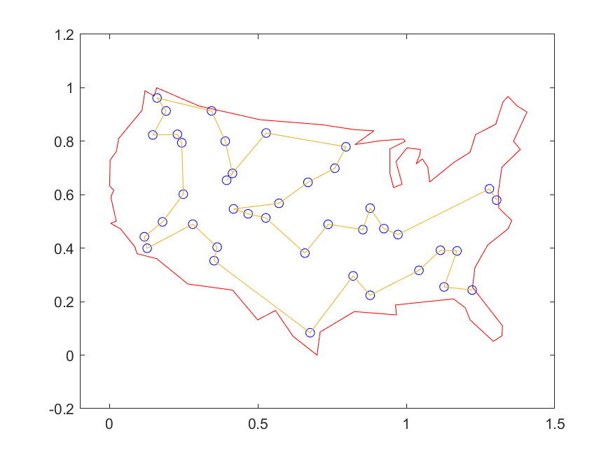

适用的范围

一个在解空间内进行搜索的优化问题。需要能够方便地对解空间进行编码。